2D Topology Optimization Example

Classic 2D Structured Meshes

In this example we will show how you can use pyFANTOM to perform minimum compliance TO on structured meshes in 2D. For this example we will perform TO on the bridge problem.

Below we detail how you can do this in a few lines of code!

Importing The Necessary Tools

First we import the tools from pyFANTOM we will be using in this example.

from pyFANTOM.CPU import(
    StructuredMesh2D, # Mesh Object for 2D Structured Meshes
    StructuredFilter2D, # Filter kernel for 2D Structured Meshes
    StructuredStiffnessKernel, # Stiffness Kernel for 2D Structured Meshes
    FiniteElement, # Finite Element Object to Setup Boundary Conditions and RHS
    CHOLMOD, CG, GMRES, MultiGrid, SPLU, SPSOLVE, # Sparse Solvers
    MinimumCompliance, # TO Problem Definition
    PGD, MMA, OC # Nonlinear Optimizers
)

from pyFANTOM.Physics import LinearElasticity # Physics Model For FEA

# Other Imports
import numpy as np
import matplotlib.pyplot as plt
from tqdm import trange

Setting Up Physics and Geometry

The first step in using pyFANTOM is defining the domain of the problem and setting up the physics for FEA.

length = 1.0
height = 0.25

# Create a physics model
physics = LinearElasticity(E=1.0, nu=1/3, thickness=1.0, type='PlaneStress')

# Create a mesh
mesh = StructuredMesh2D(nx=256, ny=64, lx=length, ly=height, physics=physics)

Setting Up The Finite Element Solver

The next step in using pyFANTOM is setting up a stiffness kernel and finite-element boundary conditions.

# Create a stiffness kernel
stiffness_kernel = StructuredStiffnessKernel(mesh=mesh)

# Create a solver
solver = CHOLMOD(kernel=stiffness_kernel) # This can be any of the sparse solvers in pyFANTOM

# Create a finite-element object
fe = FiniteElement(mesh=mesh, kernel=stiffness_kernel, solver=solver)

# Visualize the problem
plt.figure(figsize=(10, 5))
fe.visualize_problem()
plt.tight_layout()
plt.axis('off')

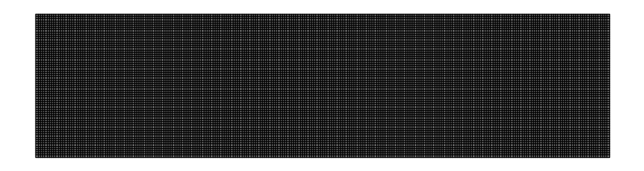
As seen above we do not have loads or boundary conditions. So now we will set this up for the bridge problem:

left_edge_nodes = np.where(mesh.nodes[:, 0] < 1e-12)[0]
right_edge_nodes = np.where(mesh.nodes[:, 0] > length - 1e-12)[0]

bottom_edge_nodes = np.where(mesh.nodes[:, 1] < 1e-12)[0]

fe.reset_dirichlet_boundary_conditions()
fe.reset_forces()
# Apply force to the bottom edge
fe.add_point_forces(
    node_ids=bottom_edge_nodes,
    positions=None,
    forces=np.array([[0.0, -1.0/len(bottom_edge_nodes)]])
)

# Apply zero displacement to the left edge and the right edge
fe.add_dirichlet_boundary_condition(
    node_ids=np.concatenate([left_edge_nodes, right_edge_nodes]), # Node IDs to apply the boundary condition to
    positions=None, # Alternative way to specify the boundary condition is to pass positions in space
    dofs=np.array([[1, 1]]), # Degrees of freedom to apply the boundary condition to
    rhs=0.0 # Value to apply the boundary condition to
)

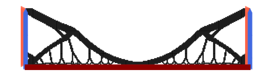
# Visualize the problem
plt.figure(figsize=(10, 5))
fe.visualize_problem()
plt.tight_layout()
# plt.autoscale(enable=True)
plt.margins(0.12)
plt.axis('off')

Setting Up TO Problem And Optimizer

Once the finite element is setup we can define the problem and optimizer to perform TO.

# Define the filter kernel for TO
filter_kernel = StructuredFilter2D(mesh=mesh, r_min=1.5)

# Define the TO problem
to_problem = MinimumCompliance(
    FE=fe,
    filter=filter_kernel,
    E_mul=[1.0], # You can pass a list of values to perform multi-material TO
    volume_fraction=[0.2], # You can pass a list of values to perform volume fraction control for each material
    void=1e-9, # You can pass a value to set void modulus
    penalty=3, # You can pass a value to set penalty factor
    #penalty_schedule = lambda p, i: (p-1)*np.round(4 * min(100, i) / 100)/4 + 1, # You can pass a function to set penalty schedule here
    heavyside= True, # You can pass a boolean to use heavyside or not
    eta=0.5, # You can pass a value to set eta - only used for heavyside
    beta=2.0, # You can pass a value to set beta, or a function of iteration to set beta schedule - only used for heavyside
)

# Define the optimizer
optimizer = PGD( # You can use any of the optimizers in pyFANTOM: OC, MMA, PGD
    problem=to_problem,
    change_tol=np.inf, # No change tolerance
    fun_tol=1e-4, # Function tolerance (convergence criterion for the optimizer)
)

Running The Optimization Loop

Now we can run the optimization loop and perform TO.

maximum_iterations = 300

Progressbar = trange(maximum_iterations, desc='Optimizer Iterations', leave=True)
objective_history = []
for i in Progressbar:
    optimizer.iter()

    Progressbar.set_postfix(
        optimizer.logs()
    )

    objective_history.append(optimizer.logs()['objective'])

    if optimizer.converged():
        print(f'Converged in {i} iterations')
        break

The optimization converged in 56 iterations with the following output:

Optimizer Iterations:  19%|█▊        | 56/300 [01:04<04:40,  1.15s/it, objective=11.6, variable change=0.936, function change=5.92e-5, iteration=58, residual=2.56e-12] Converged in 56 iterations

Now we can visualize the resulting topology:

plt.figure(figsize=(10, 5))
to_problem.visualize_solution()
plt.tight_layout()
# plt.autoscale(enable=True)
plt.margins(0.1)
plt.axis('off')

Running on GPU

The exact same problem can be run on GPU by just switching the backend.

A few notes on CUDA back-ends: - In general the only exact solver available for CUDA is SPSOLVE, but in general for structured meshes the Multi-Grid solver with our custom CUDA kernels is the fastest solver on GPU. - The CUDA backend uses cupy, however, the inputs to the FE class can be numpy arrays.

from pyFANTOM.CUDA import(
    StructuredMesh2D, # Mesh Object for 2D Structured Meshes
    StructuredFilter2D, # Filter kernel for 2D Structured Meshes
    StructuredStiffnessKernel, # Stiffness Kernel for 2D Structured Meshes
    FiniteElement, # Finite Element Object to Setup Boundary Conditions and RHS
    CG, GMRES, MultiGrid, SPSOLVE, # Sparse Solvers
    MinimumCompliance, # TO Problem Definition
    PGD, MMA, OC # Nonlinear Optimizers
)

from pyFANTOM.Physics import LinearElasticity # Physics Model For FEA

# Other Imports
import numpy as np
import matplotlib.pyplot as plt
from tqdm import trange


length = 1.0
height = 0.25

# Create a physics model
physics = LinearElasticity(E=1.0, nu=1/3, thickness=1.0, type='PlaneStress')

# Create a mesh
mesh = StructuredMesh2D(nx=256, ny=64, lx=length, ly=height, physics=physics)

# Create a stiffness kernel
stiffness_kernel = StructuredStiffnessKernel(mesh = mesh)

# Create a solver
solver = MultiGrid(
    mesh=mesh,
    kernel=stiffness_kernel,
    maxiter=200,
    tol=1e-4,
    n_level=3,
    cycle='W',
    w_level=1
)

# Create a finite-element object
fe = FiniteElement(mesh=mesh, kernel=stiffness_kernel, solver=solver)

left_edge_nodes = np.where(mesh.nodes[:, 0] < 1e-12)[0]
right_edge_nodes = np.where(mesh.nodes[:, 0] > length - 1e-12)[0]

bottom_edge_nodes = np.where(mesh.nodes[:, 1] < 1e-12)[0]

fe.reset_dirichlet_boundary_conditions()
fe.reset_forces()
# Apply force to the bottom edge
fe.add_point_forces(
    node_ids=bottom_edge_nodes,
    positions=None,
    forces=np.array([[0.0, -1.0/len(bottom_edge_nodes)]])
)

# Apply zero displacement to the left edge and the right edge
fe.add_dirichlet_boundary_condition(
    node_ids=np.concatenate([left_edge_nodes, right_edge_nodes]), # Node IDs to apply the boundary condition to
    positions=None, # Alternative way to specify the boundary condition is to pass positions in space
    dofs=np.array([[1, 1]]), # Degrees of freedom to apply the boundary condition to
    rhs=0.0 # Value to apply the boundary condition to
)

# Define the filter kernel for TO
filter_kernel = StructuredFilter2D(mesh=mesh, r_min=1.5)

# Define the TO problem
to_problem = MinimumCompliance(
    FE=fe,
    filter=filter_kernel,
    E_mul=[1.0], # You can pass a list of values to perform multi-material TO
    volume_fraction=[0.2], # You can pass a list of values to perform volume fraction control for each material
    void=1e-9, # You can pass a value to set void modulus
    penalty=3, # You can pass a value to set penalty factor
    #penalty_schedule = lambda p, i: (p-1)*np.round(4 * min(100, i) / 100)/4 + 1, # You can pass a function to set penalty schedule here
    heavyside= True, # You can pass a boolean to use heavyside or not
    eta=0.5, # You can pass a value to set eta - only used for heavyside
    beta=2.0, # You can pass a value to set beta, or a function of iteration to set beta schedule - only used for heavyside
)

# Define the optimizer
optimizer = PGD( # You can use any of the optimizers in pyFANTOM: OC, MMA, PGD
    problem=to_problem,
    change_tol=np.inf, # No change tolerance
    fun_tol=1e-4, # Function tolerance (convergence criterion for the optimizer)
)

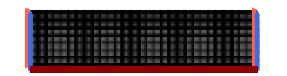
# Visualize the problem
plt.figure(figsize=(10, 5))
fe.visualize_problem()
plt.tight_layout()
# plt.autoscale(enable=True)
plt.margins(0.12)
plt.axis('off')

maximum_iterations = 300

Progressbar = trange(maximum_iterations, desc='Optimizer Iterations', leave=True)
objective_history = []
for i in Progressbar:
    optimizer.iter()

    Progressbar.set_postfix(
        optimizer.logs()
    )

    objective_history.append(optimizer.logs()['objective'])

    if optimizer.converged():
        print(f'Converged in {i} iterations')
        break

The GPU optimization converged in 43 iterations:

Optimizer Iterations:  14%|█▍        | 43/300 [00:09<00:55,  4.63it/s, objective=11.7, variable change=2, function change=2.32e-5, iteration=45, residual=8.85e-5]     Converged in 43 iterations

plt.figure(figsize=(10, 5))
to_problem.visualize_solution()
plt.tight_layout()
# plt.autoscale(enable=True)
plt.margins(0.1)
plt.axis('off')

Unstructured Meshes

pyFANTOM also supports unstructured meshes for topology optimization. Below we will use pygmesh to mesh a 2D model and perform TO on it.

NOTE: - This is a toy problem to represent the capabilities of the package not a real-world problem. - The Multi-Grid solver which is the most efficient way to solve the FEA problem is only available for structured meshes. So you may want to consider voxelizing geometry in some cases.

from pyFANTOM.CPU import(
    GeneralMesh, # Mesh Object for Unstructured Meshes
    GeneralFilter, # Filter kernel for Unstructured Meshes
    GeneralStiffnessKernel, UniformStiffnessKernel, # Stiffness Kernel for Unstructured Meshes
    FiniteElement, # Finite Element Object to Setup Boundary Conditions and RHS
    CHOLMOD, CG, GMRES, MultiGrid, SPLU, SPSOLVE, # Sparse Solvers
    MinimumCompliance, # TO Problem Definition
    PGD, MMA, OC # Nonlinear Optimizers
)

from pyFANTOM.Physics import LinearElasticity # Physics Model For FEA

import pygmsh

# Other Imports
import numpy as np
import matplotlib.pyplot as plt
from tqdm import trange

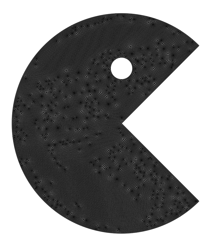
Create A Pac-Man Mesh

Below we will make a toy problem mesh using pygmesh.

# Unstructured Uniform Mesh generate on a random domain
with pygmsh.geo.Geometry(['-setnumber', 'Mesh.Algorithm', '6',
                          '-setnumber', 'Mesh.RecombinationAlgorithm', '3',
                          '-setnumber', 'Mesh.RecombineAll', '1',
                          '-setnumber', 'Mesh.SaveWithoutOrphans', '1']) as geom:
    # Pacman parameters
    body_center = [0.5, 0.5, 0.0]
    body_radius = 0.5
    mouth_angle = 45  # Half-angle for the mouth (in degrees)
    eye_center = [0.5, 0.75, 0.0]
    eye_radius = 0.05

    # Define the mouth as a wedge
    p1 = geom.add_point(
        [
            body_center[0] + body_radius * np.cos(-np.pi/4),
            body_center[1] + body_radius * np.sin(-np.pi/4),
            0.0,
        ],
        mesh_size = 0.005
    )
    p2 = geom.add_point(
        [
            body_center[0] + body_radius * np.cos(np.pi/4),
            body_center[1] + body_radius * np.sin(np.pi/4),
            0.0,
        ],
        mesh_size = 0.005
    )
    p3 = geom.add_point(
        [
            0.0,
            0.5,
            0.0,
        ],
        mesh_size = 0.005
    )
    center_point = geom.add_point(body_center, mesh_size = 0.005)

    mouth_line1 = geom.add_line(center_point, p2)
    mouth_line2 = geom.add_line(p1, center_point)
    arc1 = geom.add_circle_arc(p2, center_point, p3)
    arc2 = geom.add_circle_arc(p3, center_point, p1)

    loop = geom.add_curve_loop([mouth_line1, arc1, arc2, mouth_line2])

    eye_center_point = geom.add_point(eye_center,
        mesh_size = 0.005)
    eye_right_point = geom.add_point([eye_center[0] + eye_radius, eye_center[1], 0.0],
        mesh_size = 0.005)
    eye_left_point = geom.add_point([eye_center[0] - eye_radius, eye_center[1], 0.0],
        mesh_size = 0.005)
    eye_arc1 = geom.add_circle_arc(eye_right_point, eye_center_point, eye_left_point,)
    eye_arc2 = geom.add_circle_arc(eye_left_point, eye_center_point, eye_right_point)

    eye_loop = geom.add_curve_loop([eye_arc1, eye_arc2])

    surface = geom.add_plane_surface(loop, holes=[eye_loop])

    # Generate the mesh
    mesh_uniform = geom.generate_mesh()

    mesh_uniform = [mesh_uniform.points[:,0:2], mesh_uniform.cells[1].data.astype(int).tolist()]

# Create a physics model
physics = LinearElasticity(E=1.0, nu=1/3, thickness=1.0, type='PlaneStress')
mesh = GeneralMesh(np.array(mesh_uniform[0]), np.array(mesh_uniform[1]), physics=physics)

# Create a stiffness kernel
if mesh.is_uniform:
    stiffness_kernel = UniformStiffnessKernel(mesh=mesh)
else:
    stiffness_kernel = GeneralStiffnessKernel(mesh=mesh)

# Create a solver
solver = CHOLMOD(kernel=stiffness_kernel)

# Create a finite-element object
fe = FiniteElement(mesh=mesh, kernel=stiffness_kernel, solver=solver)

# Visualize the mesh
plt.figure(figsize=(10, 10))
fe.visualize_problem()
plt.tight_layout()
plt.axis('off')

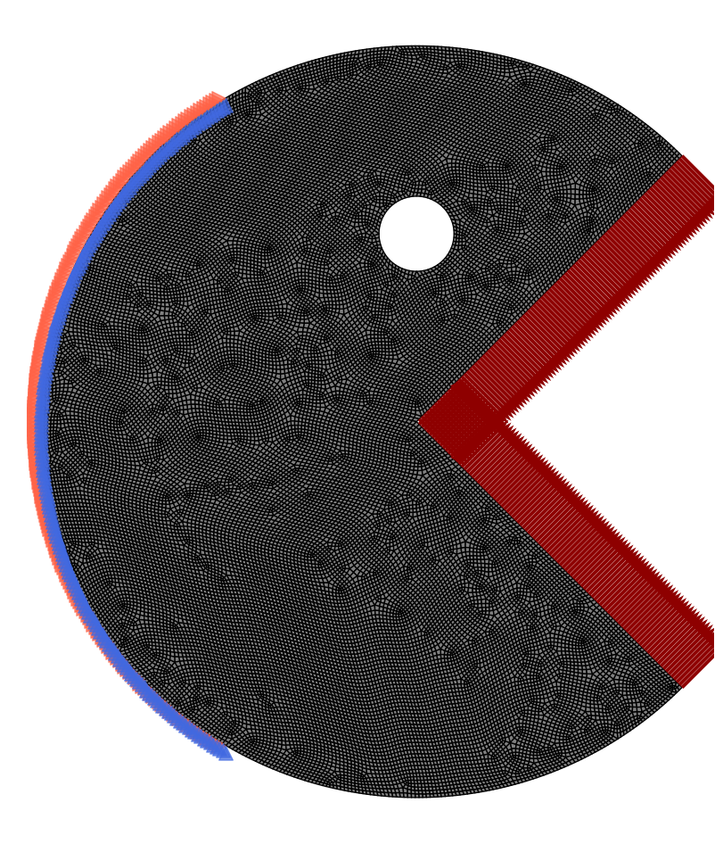
Now we will setup boundary conditions for this toy problem:

fe.reset_dirichlet_boundary_conditions()
fe.reset_forces()

# find nodes on the boundary of the packman circle
bc_nodes = np.isclose(np.linalg.norm(mesh.nodes[:,0:2] - np.array([0.5,0.5]), axis=1),0.5)
bc_nodes = np.logical_and(bc_nodes, mesh.nodes[:,0] < 0.25)
bc_nodes = np.where(bc_nodes)[0]

fe.add_dirichlet_boundary_condition(
    node_ids=bc_nodes,
    positions=None,
    dofs=np.array([[1, 1]]),
    rhs=0.0
)

# apply load at the mouth of the packman
upper_mouth = np.logical_and(np.isclose(np.abs(np.dot(mesh.nodes,np.array([-1,1]))),0), mesh.nodes[:,0] > 0.5)
force_node = np.where(upper_mouth)[0]
force_nodes = force_node[np.isin(force_node, bc_nodes, invert=True)]
force = np.array([[1,-1]])/force_nodes.shape[0]/4 # Broadcastable, If needed you can provide one for each point

fe.add_point_forces(
    node_ids=force_nodes,
    positions=None,
    forces=force
)

lower_mouth = np.logical_and(np.isclose(np.abs(np.dot(mesh.nodes,np.array([1,1]))),1.0), mesh.nodes[:,0] > 0.5)
force_node = np.where(lower_mouth)[0]
force_nodes = force_node[np.isin(force_node, bc_nodes, invert=True)]
force = np.array([[1,1]])/force_nodes.shape[0]/4 # Broadcastable, If needed you can provide one for each point

fe.add_point_forces(
    node_ids=force_nodes,
    positions=None,
    forces=force
)

# Visualize the problem
plt.figure(figsize=(10, 10))
fe.visualize_problem()
plt.tight_layout()
plt.axis('off')

Now we can just setup the problem and optimizer like before:

# Define the filter kernel for TO
filter_kernel = GeneralFilter(mesh=mesh, r_min=2.0 * 0.005) # In general cases r_min is mesh space, not scaled by mesh size be cassreful!

# Define the TO problem
to_problem = MinimumCompliance(
    FE=fe,
    filter=filter_kernel,
    E_mul=[1.0], # You can pass a list of values to perform multi-material TO
    volume_fraction=[0.25], # You can pass a list of values to perform volume fraction control for each material
    void=1e-9, # You can pass a value to set void modulus
    penalty=3, # You can pass a value to set penalty factor
    #penalty_schedule = lambda p, i: (p-1)*np.round(4 * min(100, i) / 100)/4 + 1, # You can pass a function to set penalty schedule here
    heavyside= True, # You can pass a boolean to use heavyside or not
    eta=0.5, # You can pass a value to set eta - only used for heavyside
    beta=2.0, # You can pass a value to set beta, or a function of iteration to set beta schedule - only used for heavyside
)

# Define the optimizer
optimizer = PGD( # You can use any of the optimizers in pyFANTOM: OC, MMA, PGD
    problem=to_problem,
    change_tol=np.inf, # No change tolerance
    fun_tol=1e-4, # Function tolerance (convergence criterion for the optimizer)
)

maximum_iterations = 300

Progressbar = trange(maximum_iterations, desc='Optimizer Iterations', leave=True)
objective_history = []
for i in Progressbar:
    optimizer.iter()

    Progressbar.set_postfix(
        optimizer.logs()
    )

    objective_history.append(optimizer.logs()['objective'])

    if optimizer.converged():
        print(f'Converged in {i} iterations')
        break

The unstructured mesh optimization converged in 198 iterations:

Optimizer Iterations:  66%|██████▌   | 198/300 [08:03<04:09,  2.44s/it, objective=1.47, variable change=0.12, function change=9.93e-5, iteration=200, residual=9.82e-13]  Converged in 198 iterations

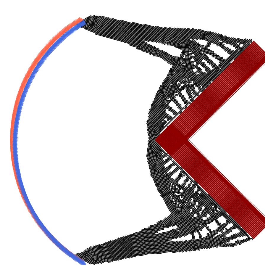
# Visualize the solution
plt.figure(figsize=(10, 10))
to_problem.visualize_solution()
plt.tight_layout()
plt.axis('off')